
Finding the Shortest Path using the Tobler Function
The following post was made trying to understand the functions withing
the gdistance R package by Jacob van Etten.
Here is the documentation of the pacakge
During the process there will by answer the following questions found GIS StackExchange:
- Working out travel time from gdistance’s conductance values in R?
- Calculating accumulated walking pace from starting location outwards using R?
- Integrating use of surface distance when calculating cumulative cost-surface based on walking pace?
Basic functioning
library(dplyr)
library(gdistance)
library(raster)
library(sf)
library(RColorBrewer)
library(mapview)
library(htmlwidgets)
library(rgeos)
library(leaflet)
Usning a randomized raster with height values, we can see the cost of moving from an starting cell. Let’s create the matrix
r <- raster(nrows=6, ncols=7,
            xmn=0, xmx=7,
            ymn=0, ymx=6,
            crs="+proj=utm +units=m")

r[] <- c(2, 2, 1, 1, 5, 5, 5,
         2, 2, 8, 8, 5, 2, 1,
         7, 1, 1, 8, 2, 2, 2,
         8, 7, 8, 8, 8, 8, 5,
         8, 8, 1, 1, 5, 3, 9,
         8, 1, 1, 2, 5, 3, 9)
Calculate CONDUCTANCE (transition) and plot with original raster:
# CONDUCTANCE: 1/mean: reciprocal to get permeability
tr <- transition(r, function(x) 1/mean(x), 8)
tr <- geoCorrection(tr, scl=FALSE)

# plot raster and conductance
par(mfrow = c(1,2), mar=c(0,0,0,5))
plot(r)
text(r)
x <- raster(tr)
plot(x)
for(i in 1:ncell(x)){
 xycoords <- xyFromCell(x, cell = i)
 value <- extract(x, xycoords)
 text(xycoords, labels = round(value, 3))
}

Now lets calculate the accumulated cost and the shortest path between cells
# Calculate accumulated cost
c1 <- c(1,6)
c2 <- c(6,2)
cost <- accCost(tr, c1)

# Shortest path
path1 <- shortestPath(tr, c1, c2, output="SpatialLines")
path2 <- shortestPath(tr, c2, c1, output="SpatialLines")

# Plots
par(mfrow=c(1,2))
# Accumulated cost
plot(cost)
text(cost)
# Shortest path
plot(cost)
plot(path1, add=TRUE, col = 'blue', lwd=5)
plot(path2, add=TRUE, col = 'red')

(un) Real example
Now we will calculate the shortest routes between 3 points using a real digital elevation model an a real walking speed function that varies with topology (slope).
First, read raster dtm and generate random points to calculate routes:
# Read raster
r <- raster("../../data/20220720/DTM.tif")

# Select random coords within the raster
set.seed(1234)
A <- coordinates(r)[sample(dim(r)[[1]]*dim(r)[[2]])[[1]],]
B <- coordinates(r)[sample(dim(r)[[1]]*dim(r)[[2]])[[1]],]
C <- coordinates(r)[sample(dim(r)[[1]]*dim(r)[[2]])[[1]],]

# coords as sf
library(data.table)
cs <- data.table(ID=c("A", "B", "C"),
                 x=c(A[[1]], B[[1]], C[[1]]),
                 y=c(A[[2]], B[[2]], C[[2]]))

# st_as_sf() ######
ps <- st_as_sf(cs, coords = c("x", "y"), crs = 25829, agr = "constant")
ps <- ps %>% mutate(x=st_coordinates(ps)[[1]], y = st_coordinates(ps)[[2]])

# plot
plot(r)
points(as_Spatial(ps))
text(st_coordinates(ps), labels = ps$ID, pos = 4)

Calculate cell differences between adjacent cells and apply the Toble’s function to correct speed:
# Calculate the height differences between cells (neet to calculate slope)
altDiff <- function(x){x[2] - x[1]}
suppressWarnings({ hd <- gdistance::transition(r, altDiff, 8, symm=FALSE) })
slope <- gdistance::geoCorrection(hd, scl=FALSE) # divide transition by distances between cells

# Calculate speed
adj <- raster::adjacent(x=r, cells=1:ncell(r), direction=8)
speed <- slope
speed[adj] <-  exp(-3.5 * abs(slope[adj] + 0.05)) # m/s

# Geocorrection divides speed by distance (i.e., cells' centers)
conduct <- gdistance::geoCorrection(speed, scl=FALSE) # conductance = speed/distance = 1/travel time
Plot of conductance:
plot(raster(conduct))
points(as_Spatial(ps))
text(st_coordinates(ps), labels = ps$ID, pos = 4)

Calculate traveltime.
This is a solution to a QGIS Stack exchange question.
Extracted from “R Package gdistance: Distances and Routes on Geographical Grids” (Jacob van Etten)
What do these values mean? The function geoCorrection divides the values in the matrix between the distance between cell centres. So, with our last command we calculated this: conductance = speed/distance This looks a lot like a measure that we are more familiar with: traveltime = distance/speed In fact, the conductance values we have calculated are the reciprocal of travel time. 1/traveltime = speed/distance = conductance
So, just invert the last formula, so: traveltime = 1/conductance
tv <- raster(conduct)
values(tv) <- 1/values(raster(conduct))
See results of traveltime
plot(tv)
points(as_Spatial(ps))
text(st_coordinates(ps), labels = ps$ID, pos = 4)

Calculate cost surface from A to the others
csA <- accCost(conduct, A)
csB <- accCost(conduct, B)
csC <- accCost(conduct, C)

#plot
par(mfrow=c(1,3))
plot(csA)
points(as_Spatial(ps))
text(st_coordinates(ps), labels = ps$ID, pos = 4)
plot(csB)
points(as_Spatial(ps))
text(st_coordinates(ps), labels = ps$ID, pos = 4)
plot(csC)
points(as_Spatial(ps))
text(st_coordinates(ps), labels = ps$ID, pos = 4)

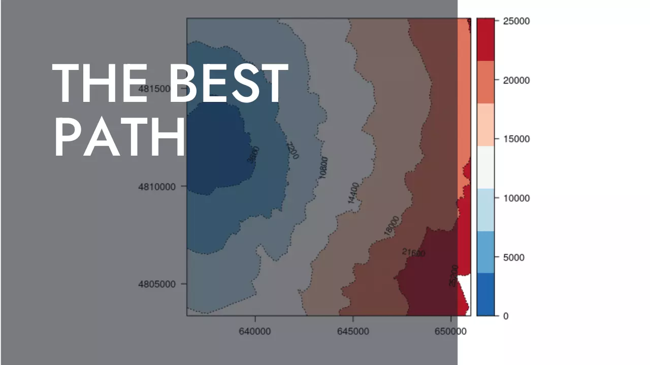
Can these results converted into isochrones ?
Here is an example of travel time from A to any other places by isochrones of an hour (3600).
library(rasterVis)
levels <- seq(min(values(csA)), max(values(csA)), 3600)
rasterVis::levelplot(csA, par.settings = BuRdTheme, margin=FALSE,
                     contour=TRUE, at = levels, lty=3,
                     labels = list(cex = 0.7), label.style = 'align')

Calculate shortest path:
AB <- shortestPath(conduct, A, B, output="SpatialLines")
AC <- shortestPath(conduct, A, C, output="SpatialLines")
BA <- shortestPath(conduct, B, A, output="SpatialLines")
BC <- shortestPath(conduct, B, C, output="SpatialLines")
CA <- shortestPath(conduct, C, A, output="SpatialLines")
CB <- shortestPath(conduct, C, B, output="SpatialLines")
Check results with mapview:
Check if results make sense
We can check results by calculating the time expended
ACdist <- st_length(st_as_sf(AC))
kmh <- 5 # normal walking speed in km/h
msv <- kmh*(1/60)*(1/60)*1000 # normal walking speed in m/s
traveltimeAC <- as.numeric(ACdist) * msv
traveltimeAC
## [1] 4542.591
tvAC <- raster::extract(csA, ps[3,])[[1]]
tvAC
## [1] 4712.175
So, in a normal pace walking, going from A to C it will take 4543 seconds, while using the tobler function time will increase to 4712 seconds. As expected, topology will increase the travel time.


